Open Access: green vs. gold, and the culture of the disconnect

Four years ago I wrote about how Open Access would be adopted if it were convenient. Polls at the time showed that few scientists actively seek to publish OA, even though many support it. Reasons given, in no particular order: aiming for journals that were not OA and high publication fees. My conclusion was that researchers will try to publish OA not from any OA ideology, but from convenience. I should have added also palpable gain (e.g.  in publication venue prestige).

So for open access week, I decided to revisit that post “The Revolution Will be Convenient“. Has anything changed since?

No and yes. In a 2014 survey of Canadian researchers, immediate Open Access received only 3.3 out of possible 100 importance points. OA publishing after an embargo period received 2.2 points. The top consideration for choosing a publication venue were impact factor (26.8 points) and journal reputation (42.9).  So in that sense, (and assuming the Canadian survey reflects the attitudes of  scientists from other countries) little has changed. While  there may be a positive attitude towards publishing immediate OA, there is little incentive to do so. Scientists want to make a splash every time they publish, but most do not seem to equate Open Access with “making a splash”. Researchers are still mostly more concerned about promotion and grant review committees reading where they published rather than growing the audience reading what they published.


“The survey suggests however, that there is a disconnect between researchers’ apparent agreement with the principle of open access (i.e., that research should be freely available to everyone) and their publishing decision criteria. Although the vast majority of researchers (83%) agree with the principle of open access, the availability of open access as a publishing option was not an important decision criterion when selecting a journal in which to publish. In this regard, availability of open access ranked 6th out of 18 possibility criteria. It was eight times less important than impact factor and thirteen times less important than journal reputation when selecting a journal” (Source)


But it seems like things are changing, although those changes are being made from the establishment rather than from the people. So not exactly a revolution: the people still overwhelmingly favor prestige over access. Increasingly, funding agencies and universities are mandating OA publication, although not immediate, author-pays “gold” open access. The mandates are mostly for self-archiving, or “green” open access.  The NIH has been mandating publication within 12 months of all NIH research. Other US Federal agencies have been directed to develop a policy for expanding access to Federally funded research by the White House Office of Science and Technology Policy. Open access mandates by funding agencies are not a done deal yet, but the wind seems to be blowing in that direction. Many journals are allowing now for self-archiving of preprints and pre-publication copies.  Green open access is convenient, free of publication charges, and mostly does not interfere with the main consideration that researchers have for publication venue: the “high profile” journal.


Graph of mandates by quarter

Growth of funder and institutional open-access mandates, Source: http://roarmap.eprints.org/


So is there a problem? Yes, several. First, embargo period. Green OA allows for an embargo period, which means that the final paper is not immediately freely available. Anyone wishing to read the latest and hopefully greatest achievements in science would still be stumped by a paywall. Of course, this goes back to the whole “who do I care who reads me?” question: researchers seem to mostly care about other researchers reading what (and where) they published. Those colleagues would mostly have access to the manuscript anyway. Second, self-archiving and preprint policies vary, even if a self-archived copy is available, it may take some effort to locate it, although Google Scholar seems to be doing a pretty good job in that department. Finally, publishers’ policy regarding preprints vary and are sometimes unclear, which can deter researchers from self-archiving lest they violate some policy.  So green is not without its shortcomings, even without an embargo period.

In the UK, a 2012 report by The Working Group on Expanding Access to Published Research Findings supported Gold OA. It discounted the Green methods for many of the reasons stated above, and recommended the author-pays, immediate publishing model.


“If green is cumbersome, messy, involves assumptions about cooperation and investment in infrastructure, and still only delivers an imperfect version of the article, and then several months after publication, surely it’s better to pay for the final version to be accessible upon publication?” (Source)


On the plus side, no-one is really arguing anymore on whether we should even publish open access. OA is here to stay, and  the questions asked today relate to degrees of accessibility and freedom to reproduce, and financial models to support OA. But the Canadian survey has brought this to the forefront:  something is wrong in a scientific culture that has turned communication into coinage, and the disconnect between the values researchers profess (overwhelmingly pro open-access), and what they actually practice (OA counts for little when choosing a publication venue), is worrying.

So great are the rewards for publishing in top academic journals that everyone games furiously – authors, editors, universities and academic publishers… (Source)


Share and Enjoy:
  • Fark
  • Digg
  • Technorati
  • del.icio.us
  • StumbleUpon
  • Facebook
  • Reddit
  • Twitter
  • FriendFeed
  • PDF
  • email
  • Print
  • Google Bookmarks

Choosing a software license

(With apologies to the memory of Elizabeth Barrett Browning)

How shall I license thee? Let me count the ways

I license thee to be free to distribute and embed

My code can be buggy, when I wrote it late last night

“While” loops have been made without a stated end

I license thee to change and modify

Most urgent need, by emacs and vi

I license thee MIT, as men strive for Right,

I license thee QPL, as they turn from Praise.

I license thee with a Python, put to use

In my old griefs, and with my postdoc’s faith.

I license thee with a license I seemed to lose

With my crashed disk, — I license thee with the BSD

Mozilla, Apache, of all my web-stuff! – and, if Stallman choose,

I shall license thee better with GPLv3.

Share and Enjoy:
  • Fark
  • Digg
  • Technorati
  • del.icio.us
  • StumbleUpon
  • Facebook
  • Reddit
  • Twitter
  • FriendFeed
  • PDF
  • email
  • Print
  • Google Bookmarks

Sequencing the frog that can save lives

TL; DR:  The genome sequence of the North American Wood Frog will tell us a lot about the genetic control of freezing and reanimating whole organisms. My friend and colleague, Dr. Andor Kiss is crowdfunding this project. If you would like to help, please go to experiment.com. You will get acknowledged by name in the paper. To learn more on why this is cool and important, read below.

Eighteen people die each day in the US waiting for an organ transplant. Every ten minutes, a person gets added to the waiting list. The need for improvement in organ donations is real.


Why are these statistics so grim? Even when a potentially good match is found (which can take months or years), there is a very short window between the time an organ is donated, and the time it can be transplanted. The maximum viability time for a human kidney is estimated at 35 hours; a liver 20, and a lung less than 10.  This time constraint also limits the availability of matching organs. Just  imagine if we could freeze and thaw organs without the risk of killing them, keeping them viable for months or even years. The time patients need to wait would be shorter, and, also, better matches may be found as the number of frozen organs increase. If we could learn to freeze organs without damaging them, we would revolutionize organ transplant in the same way refrigeration and freezing revolutionized the food industry. Today, however, freezing organs is not an option: once an organ is frozen, there is irreversible and widespread damage from the formation of ice crystals.  Cells shrivel and collapse, blood vessels disintegrate, connective tissue rips apart.

But there are animals that can freeze and re-animate multiple times. In fact, if you live in the northern parts of  North America, you have probably seen one, and almost surely heard it: the North American Wood Frog. The Wood Frog can freeze solid and then thaw – multiple times – with no ill effect.  During this freeze event, the frog dumps glucose (a sugar) and high levels of urea (an acid normally found in urine)  into its bloodstream. The glucose pulls water out of the cells and causes ice to freeze outside of the cells – a type of cryo-dehydration. This is to prevent ice forming inside the cells, where it would cause irreparable damage. The urea is thought to do two things – one, it also protects the cells integrity from damage, and two, it helps slow down the frog’s metabolism. The fact that the frog can freeze in and of itself is pretty spectacular – no heartbeat, no brain activity, no movement.  When it thaws, the animal spontaneously reanimates.


What seems even more bizarre about this animal is that once the frog is acclimated to summer, freezing it will simply kill it. We think that there is some sort of seasonal trigger for winter and the possibility of freezing. There must therefore be a change of gene expression between the summer and winter frogs. One could think of this animal as its own experimental control! So to understand how the Wood Frog can survive freezing, we just pick frogs from different seasons, and see the difference in RNA expression. This can clue us into what makes a freeze-adapted frog different than a non-freeze adapted one. Andor has actually been doing that, and will be talking about it next week at the American Physiological Society Meeting in San Diego (if you’re there, walk up to him and say “hi”).  But what Andor doesn’t have, is a good reference genome. Nothing close to the Wood Frog has been sequenced yet. Xenopus is a genus of frogs used in laboratories whose genomes have been sequeenced. But as a reference for Wood Frog, the Xenopus genomes aren’t good — the two species are too far apart.

Even more interesting,  having the genome of the wood frog will enable studies of the different epigenetic patterns between summer and winter frogs. The control of gene expression is ultimately what Andor is interested in sorting out, and it’s likely that the epigenetics is involved: changes in the DNA that are not in the actual sequence, (like methylation) and affect the production of RNA and proteins.   Additionally, because we don’t know the wood frog genome yet, we may find gene family expansions and contractions, novel genes that impart the freeze tolerance to the animal that we cannot possibly predict using a hypothesis driven approach.

And it can all be done relatively cheaply. For less than $4,000 (which is what Andor is asking for), one can do a vertebrate genome.  That makes it feasible for a single researcher to (a)  build the library, and (b) having the sequencing done. Annotation, of course, is another story, but we are planning a jamboree for that. Stay tuned.

Interested? The project is not too expensive, only $4,000! Any little bit helps a lot. Please go to the science crowdfunding site experiment.com, and give something.  You will get acknowledged by name in the paper as part of the “Wood Frog Sequencing Consortium”.  Thank you!


Share and Enjoy:
  • Fark
  • Digg
  • Technorati
  • del.icio.us
  • StumbleUpon
  • Facebook
  • Reddit
  • Twitter
  • FriendFeed
  • PDF
  • email
  • Print
  • Google Bookmarks

Work jargon scientists should have

Fakeference invitation: an email from Nancy, Sally or June, inviting you, for the second time (“perhaps you didn’t get my first invitation, there may be something wrong with my email”) to speak at a conference. The meeting has  5-10 Nobel laureates listed as invited speakers, and covers everything in science, from quantum mechanics to fish breeding. Needless to say, there is no meeting.

Fauxpen access: when a published offers “open access” publication, but not really. The paper is not under Creative Commons, the publisher still holds the copyright. Doesn’t stop them from charging you $4,000.

Grantxiety: that time between the moment you hear that your grant has scored well, and the moment you hear that it is still too low to be funded.

LinkedWho: an invitation from someone you don’t know to join on LinkedIn.

Paper turfing: when you refuse a request to review a manuscript, because the abstract is so poorly written you don’t even want to think what it would be like to slog through the whole paper.

PCWave: (rhymes with “PCA”): someone showing a principal components analysis chart at a seminar, furiously waving their hands around the data points to convince the audience they are clustered in some meaningful way.

Spamdoc: an email beginning with “Dear esteemed professor”, continues to list a a science biography that has no relevance to the research you do, and ends with a request to join your lab.

Starer bars: uncategorized, unannotated error bars in a graph. Are these SD, SE, CI or what? I don’t know, I guess I’ll just stare.

Travel dead zone: too far to drive, too near to fly (does not apply to countries that have good trains).

Virtual absence : taking your laptop to a coffee shop, activating the away message on your email and not answering the phone because you want to get some work done.

Virtual presence: being at a remote conference but answering work emails and Skype calls any time. Including 3am.

Workminar: when you go to a seminar for politeness sake, but take your laptop and work furiously through it because the grant deadline is tomorrow.


Share and Enjoy:
  • Fark
  • Digg
  • Technorati
  • del.icio.us
  • StumbleUpon
  • Facebook
  • Reddit
  • Twitter
  • FriendFeed
  • PDF
  • email
  • Print
  • Google Bookmarks

Estimating how much we don’t know

ResearchBlogging.org

Or: “Estimating how much we don’t know, and how much it can hurt us”.

This post is about a paper I published recently with Predrag Radivojac’s group at Indiana University, who lead the study.

One of the main activities I’m involved with is CAFA,* the critical assessment of function annotations.   The general idea of CAFA is to assess how well protein function prediction algorithms work.

Why is it important to do that? Because today most of our understanding of what genes do comes from computational predictions, rather than actual experiments. For almost any given gene that is sequenced, its function is determined by putting its sequence through one or more function annotation algorithms. Computational annotation is cheaper and more feasible than cloning, translating, and assaying the gene product (typically a protein) to find out exactly what it does. Experiments can be long, expensive and,  in many cases, impossible to perform.


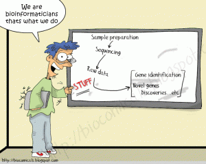
stuff

But, by resorting to computational annotation of the function of proteins, we need to know how well can these algorithms actually perform. Enter CAFA, of which I have written before. CAFA is a community challenge that assesses the performance of  protein function prediction algorithms.

How does the CAFA challenge work? Well, briefly:

1. Target selection: we select a large number of proteins from SwissProt, UniProt-GOA and other databases. Those proteins have no experimental annotations, only computational ones. Those are the prediction targets.

2. Prediction phase: we publish the targets. Participating CAFA teams now have four months to provide their own functional annotations, using the Gene Ontology, a controlled vocabulary describing protein functions.

3. Growth phase: after four months, we close the predictions, and wait for another six months, or so. During those six months, some of the targets acquire experimentally-validated annotations. This typically means that biocurators have associated some of these proteins with papers for which experimental data have been provided, we call the targets that have been experimentally annotated during this phase benchmarks. Typically, the benchmarks are a small fraction of the targets. But since we pick about 100,000 targets, even a small fraction comprise a few hundred benchmarks, which is enough to assess how well programs match these proteins to their functions.

4. Assessment: we now use the benchmark proteins to assess how well the predictions are doing. We look at the GO terms assigned to the benchmarks, and compare them with the GO terms which the predictors gave.

Sounds good, what’s the problem then?

Well, there are a few, as there are with any methods challenge. For one, who’s to say that the metrics we use to assess algorithm prediction quality are the best ones? To address that, we actually use several metrics, but there are some we don’t use. Our AFP meetings always have very lively discussions about these metrics. No bloody noses yet, but pretty damn close.

Bu the issue I would like to talk about here is how much can we know at the time of the assessment? Suppose someone predicts that the target protein “X” is a kinase. Protein “X” happened to be experimentally annotated during the growth phase, so now it is a benchmark. However, it was not annotated as a kinase. So the prediction that “A” is a kinase is considered to be, at the assessment, a false positive. But is it really? Suppose that a year later, someone does discover that X is a kinase. The prediction was correct after all, but because we did not know ti at the time, we dinged that method a year ago when we shouldn’t have. The same goes for the converse: suppose “X” was not predicted to be a kinase, and was also assessed not to be a kinase. Two  years later, “X” is found out to be a kinase. In this case, not predicting a kinase function  for “X” was a false negative prediction. And we gave a free pass to the methods that did not catch that false negative. The figure blow illustrates that at time “A” we have an incomplete knowledge, when compared to a later time “B”.

F1.large

At the time of assessment (A), we claim to know all the false positives(fp) , false negatives (fn)  true positives (tp) and true negatives (tn) of the CAFA predictions. But then at a later time, (B), we may discover errors in our assessment as we gain more data. At time (B), α is the number of true negatives we did not know of at time (A), and β is the number of false positives we did not know of at time A. The sum of both errors is δ. Source: http://bioinformatics.oxfordjournals.org/content/30/17/i609.abstract

So how many of these false false-positives and false false-negatives are there? Putting it another way, by how much does the missing information at any given time affect our ability to accurately assess the accuracy of the function prediction algorithms? If we assess an algorithm today only to discover that are assessment is wrong a year from now, our assessment is not worth much, is it?

To answer this question, I first have to explain how we assess CAFA predictions. There are two chief ways we do that. First, there is a method using precision (pr) and recall (rc). Precision/recall assessments are quite common when assessing the performance of prediction programs.

$latex pr=\frac{tp}{tp+fp}&s=1$    $latex rc=\frac{tp}{tp+fn}&s=1$

The precision is the number of correct predictions out of all predictions, true and false. Recall is the number of correct predictions out of all known true annotations. (tp: true positives; fp: false positives; fn: false negatives). We can use the harmonic mean of precision and recall to boil them down to one number also known as F1:

$latex F_1 = 2\times \frac{pr\times rc}{pr+rc}&s=1 $

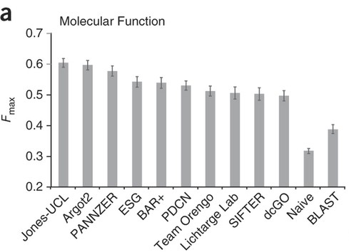
The F1 is one metric we use to rank performance in CAFA. If a prediction is perfect, i.e. no false positives or false negatives, fp=0, fn=0 then the precision equals 1, the recall equals 1 and F1=1. On the other hand, if there are no true positives (tp=0 that is, the method didn’t get anything right), then F1 =0. between these two extremes lie the spectrum of  scores of methods predicting in CAFA. Here is how well the top-scoring methods did in CAFA1:

nmeth.2340-F2

These are the maximum F1 scores for all methods in the first CAFA. BLAST was used as a baseline, and is shown on the right. Taken from: http://www.nature.com/nmeth/journal/v10/n3/full/nmeth.2340.html


But the F1 (or rather Fmax, the maximum F1 for each method) given here is for time (A), when we first assess CAFA. But at time (A) our knowledge is incomplete. At time (B) we know more! We have some idea of the alpha and beta errors we made.(At later time points, C etc. we will know more still).

OK, so let’s rescore the methods at time B, call this new score F’1. First, the new precision and recall, pr‘ and rc‘ at time (B), when we are wiser than (or at least more knowledgeable of our errors at)  time (A).

$latex pr’=\frac{tp+\beta}{tp+fp}&s=1$      $latex rc’=\frac{tp+\beta}{tp+fn+\alpha+\beta}&s=1$

So F’1 is:

$latex F’_1= \frac{2\times tp+\beta}{2tp+fp+fn+\alpha+\beta}&s=1$

So what? Bear with me a bit longer.  We now formalized the F1 (at the time of our first assessment) and F’1 (at some later time when we know more and recognize our α  and  β errors). What we are interested in is whether the differences between F1 and F’1 are significant. We know that pr’pr because beta > 0. The change in precision is

$latex \Delta pr= pr’-pr= \frac{\beta}{tp+fp}$

So the precision can only grow, and the more false positives we discover to be true positives at time (B), the better our precision gets. OK, so when we deal with precision, having  missing information on false negatives at time (A) is bad once we have more knowledge at time (B).

But what about recall and missing information on false positives? After all, F1 is a product of both precision and recall.

With recall, the story is slightly different. When rc‘ is the recall on the new annotations.

$latex rc’=\frac{\beta}{\alpha+\beta}&s=1$

I won’t get into the details here, you can see the full derivation in the paper (or work it out for yourself), but the bottom line is:

$latex \Delta F_1

\begin{cases}

\ge 0 & \text{if } rc’\ge \frac{1}{2}F_1 \\

<0 & \text{otherwise}
\end{cases}&s=1$

This is a surprising finding because only if rc’ is greater than half of the F1 will the F’1 > F1 ( that is, ΔF1>0)
1 does not depend directly on precision, only on recall!

So the F1 measure is quite robust to changes for prediction tools operating in high precision but low recall areas, which is characteristic of many of the tools participating in CAFA. The study also shows that, on real protein data, changes in F1 are not that large over time.

To be fair, the other metric that we use in CAFA, semantic distance, is more sensitive to varying values of δ. But even then the error rate is low, and we can at estimate it using studies of predictions over previous years. Our study also has simulations, playing around with α and β values to see how much we can aggravate changes in F1 and semantic distance.

Bottom line: missing information will always give us some error in the way we assess function prediction programs. But we can at least estimate the extent of the error and, under realistic conditions, the error rate is acceptably low. Making decisions when you know you don’t have enough data is a toughie, and is a much-studied problem in machine learning and game theory. Here we quantified this problem for CAFA. At least in our case, what we don’t know can hurt us, but we can estimate the level of hurt (misassessing algorithm accuracy), and it doesn’t really hurt. Much.


Jiang, Y., Clark, W., Friedberg, I., & Radivojac, P. (2014). The impact of incomplete knowledge on the evaluation of protein function prediction: a structured-output learning perspective Bioinformatics, 30 (17) DOI: 10.1093/bioinformatics/btu472

(*For all you Hebrew speakers sniggering out there — yes, the acronym is, purposefully, the Hebrew slang for “slap” כאפה).


Share and Enjoy:
  • Fark
  • Digg
  • Technorati
  • del.icio.us
  • StumbleUpon
  • Facebook
  • Reddit
  • Twitter
  • FriendFeed
  • PDF
  • email
  • Print
  • Google Bookmarks

My PLoS-ONE Academic Editor Activity Summary

I recently received an email from PLoS-ONE summarizing my editorial activity for the first half of 2014. That’s a good thing: for one, I’m terrible at keeping track of all my service activities, and this helps in keeping them straight for my own annual activities report for my university. Second, I can see how I fare vs. other editors, and how well I do generally. Looking at the report below, seems like I’m less active in the number of submissions than average I processed in this period. I am pretty efficient in finding reviewers, and seems like I end up  accepting all papers! (although those were only 2 papers at this time).  Time on my desk is about average, although I am slower in the time taken from when the revision is returned to when I make a decision. That’s probably because, unlike when I accept a paper to edit I know I have some spare time, revisions tend to come, frustratingly, when I’m trying to beat a grant deadline, during busy course exam periods, or once during my (rare) vacation time.

Overall, this is a great service PLoS-ONE provides its editors. Good work, Damian Pattinson and the rest!


Editor: Iddo Friedberg, Academic Editor

Time Period: January 1 – June 30, 2014

Join Date: 3/13/2009

My Metrics Board Avg (mean) Quartile
Number of final decisions: 2 5.78 4
Monthly avg: 0.33 .98  –
Number of first decisions: 1 5.79 4
Number currently out for revision: 1 1.34  –
Total decisions: 4 11.26 3
My Metrics Board Avg (mean) Quartile
Acceptance rate: 100% 66%  –
Efficiency of reviewer selection: 71% 44% 1
My Metrics My Median Board Avg (mean) Board Avg (median) Quartile
Avg total editorial time: 100 100 97.69 80 3
Avg time on my desk: 39.50 39.50 23.4 16 4
Percent my time to total editorial time: 39.50%  – 25% 21.63% 4
Avg time to 1st decision: 29 29 32.93 28 2
Avg time from first revision returned to final decision: 32 32 34 21 3

Definitions and abbreviations:

Quartiles: Quartiles (Q1-Q4) were calculated using standard descriptive statistics on the data set for each metric. Here, Q1 = 75-100%; Q2 = 50-75%; Q3 = 25-50%; and Q4 = 0-25%.

Number of final decisions: Total number of Academic Editor final decisions (accept or reject) within the defined time period.
Average per month: “Number of final decisions” (above), divided by the number of months covered.
Minimum: 12 final decisions per year or 6 decisions over the course of six months. Standard: 2-3 final decisions per month.
Number of first decisions: Total number of Academic Editor first decisions within the defined time period, excluding first decisions to accept or reject.

Number currently out for revision: Number of submissions with Academic Editor revision decisions awaiting author resubmission at the time when the data is retrieved.
Total decisions rendered: Total number of Academic Editor final decisions of any kind (accept, reject, major revision, minor revision) within the defined time period.

Acceptance rate: The total number of accepts divided by the total number of final decisions. PLOS ONE’s historical average has been around 70%. Very high or low acceptance rates may indicate decision-making standards not in keeping with the PLOS ONE publication criteria.
Efficiency of reviewer selection: The total number of reviews completed divided by the number of invitations.Standard: 5 invitations issued; 2 completed reviews returned.

Total editorial time. Average (mean and median) total editorial time in calendar days that each manuscript spends in the editorial process from Academic Editor assignment to final decision.
Time on my desk: “Total editorial time” (above), excluding time with the authors, journal office and reviewers, when time with reviewers is defined as the period between the first reviewer accepting the invitation and the final review being returned.
Percent of my time to total editorial time: The time on the editor’s desk divided by the total editorial time, shown as a percentage.

Time to 1st decision: Average (mean and median) total editorial time in calendar days that each manuscript spends in the editorial process from Academic Editor assignment to first decision.
Avg time from 1st revision returned to final decision: Average (mean and median) time in calendar days from a manuscript’s being returned to the Academic Editor following an initial revision, to the final decision being reached, including any subsequent review and author revision periods that may occur.

PLOS ONE Editorial Board
Share and Enjoy:
  • Fark
  • Digg
  • Technorati
  • del.icio.us
  • StumbleUpon
  • Facebook
  • Reddit
  • Twitter
  • FriendFeed
  • PDF
  • email
  • Print
  • Google Bookmarks

Mozilla does scientific matchmaking between programmers and researchers

Mozilla Science Labs are looking top pair programmers and scientists. If you are a scientist in need of a programmer,  read the following, and then go to the website to see how to take it further. Thanks to Miami University’s Office for Advancement of Research and Scholarship  for bringing this to my attention.


Interdisciplinary Programming is looking for research projects to participate in a pilot study on bringing together the scientific and developer communities to work together on common problems to help further science on the web.  This pilot will be run with the Mozilla Science Lab as a means of testing out new ways for the open science and open source community to get their hands dirty and contribute. The pilot is open to coders both within the research enterprise as well as those outside, and for all skill levels.

In this study, we’ll work to break accepted projects down to digestible tasks (think bug reports or github issues) for others to contribute to or offer guidance on. Projects can be small to mid-scale – the key here is to show how we can involve the global research and development community in furthering science on the web, while testing what the right level of engagement is.  Any research-oriented software development project is eligible, with special consideration given to projects that further open, collaborative, reproducible research, and reusable tools and technology for open science.

Candidate research projects should:

  • Have a clearly stated and specific goal to achieve or problem to solve in software.
  • Be directly relevant to your ongoing or shortly upcoming research.
  • Require code that is sharable and reusable, with preference given to open source projects.
  • Science team should be prepared to communicate regularly with the software team.

Interdisciplinary Programming was the brainchild of Angelina Fabbro (Mozilla) and myself (Bill Mills, TRIUMF) that came about when we realized the rich opportunities for cross-pollination between the fields of software development and basic research.   When I was a doctoral student writing analysis software for the Large Hadron Collider’s ATLAS experiment, I got to participate in one of the most exciting experiments in physics today – which made it all the more heartbreaking to watch how much precious time vanished into struggling with unusable software, and how many opportunities for great ideas had to be abandoned while we wrestled with software problems that should have been helping us instead of holding us back.  If we could only capture some of the coding expertise that was out there, surely our grievously limited budgets and staff could reach far further, and do so much more.

Later, I had the great good fortune to be charged with building the user interface for TRIUMF’s upcoming GRIFFIN experiment, launching this month; thanks to Angelina, this was a watershed moment in realizing what research could do if it teamed up with the web.  Angelina taught me about the incredibly rich thought the web community had in the spheres of usability, interaction design, and user experience; even my amature first steps in this world allowed GRIFFIN to produce a powerful, elegant, web-based UI that was strides ahead of what we had before.  But what really struck me, was the incredible enthusiasm coders had for research.  Angelina and I spoke about our plans for Interdisciplinary Programming on the JavaScript conference circuit in late 2013, and the response was overwhelming; coders were keen to contribute ideas, participate in the discussion and even get their hands dirty with contributions to the fields that excited them; and if I could push GRIFFIN ahead just by having a peek at what web developers were doing, what could we achieve if we welcomed professional coders to the realm of research in numbers?  The moment is now to start studying what we can do together.

We’ll be posting projects in early July 2014, due to conclude no later than December 2014 (shorter projects also welcome); projects anticipated to fit this scope will be given priority.  In addition, the research teams should be prepared to answer a few short questions on how they feel the project is going every month or so.  Interested participants should send project details to the team at mills.wj@gmail.com by June 27, 2014.


Share and Enjoy:
  • Fark
  • Digg
  • Technorati
  • del.icio.us
  • StumbleUpon
  • Facebook
  • Reddit
  • Twitter
  • FriendFeed
  • PDF
  • email
  • Print
  • Google Bookmarks

Friday Odds and Ends

So things have been busy in non-blog land. Putting together a tenure packet, some travel, teaching, and oh yes, even science. So no insightful post here, just some odds and ends I collected, in no particular order:

  • There are quite a few species named after famous people: alive, dead, real or fictional.  Wikipedia has a list.  My favorite are a golden bottom horsefly named after Beyonce; a beetle, A. schwarzennegrinamed after “the actor, Arnold Schwarzenegger, in reference to the markedly developed (biceps-like) middle femora of the males of this species reminiscent of the actor’s physique. (paper)” and a Trilobite named after Han Solo.

Arnoldv2

  • Speaking of nomenclature, meet Boops boops.
  • The Pentagon has a contingency plan for the zombie apocalypse. I feel safer already.
    Monstra_promo1
  • Are the Steven Moffat episodes of Dr. Who more sexist than those written by Russel T. Davies? A BYU student attempts to answer this question. Nice infographic. One could argue that any TV show with a powerful male alien constantly demonstrating his superiority to his female sidekick  is somewhat inherently sexist, or at least can easily go that way regardless of script writer. But see also here.
Sexist?

Sexist?

  • This post articulates my sentiments on Why Python?
Share and Enjoy:
  • Fark
  • Digg
  • Technorati
  • del.icio.us
  • StumbleUpon
  • Facebook
  • Reddit
  • Twitter
  • FriendFeed
  • PDF
  • email
  • Print
  • Google Bookmarks

The genome of nerds

What makes a nerd a nerd? The stereotype is that of someone with a high intelligence, coupled with  social awkwardness and a wardrobe that may alert the fashion police. Now scientists think they may found the genomic links to these traits.

There was always a strong suspicion of a genetic component in people that are highly skilled in certain areas of engineering and sciences. Now we think that may be due to a particular type of viral infection.  We know that human endogenous retroviruses (HERVs) make up about 8% of the human genome (that’s more than our genes, really).  But what we don’t know is how they affect us, if at all. We think we do now. Specifically, a comprehensive study of human genomes from the 10,000 genome project has linked certain retroviral markers with education levels, certain vocations, and to a smaller extent, personal income. The result: programmers, engineers,  scientists (especially physicists, statisticians and mathematicians) all had specific HERV markers not found in the general populace. Some of these markers were located next to genes coding for proteins located in the frontal lobe: the brain area associated with problem-solving.

blood-blood-blood-VIRUS

Nerd carriers?


But even more so, the overall number of HERV markers those people  was considerably smaller: sometimes less than 4%, almost half of that of the general populace. Since HERV markers are generally associated with sexually transmitted viruses this finding led the researchers to hypothesize that the early hominid ancestors of the “nerd” populace tended to mate less than the general populace. Leading to fewer HERV markers, but somehow to a more specific selection for the “brainy” traits. This would also explain the stereotypical “bright but shy” nerd.

Really interesting study, and you can read more about it  here


Share and Enjoy:
  • Fark
  • Digg
  • Technorati
  • del.icio.us
  • StumbleUpon
  • Facebook
  • Reddit
  • Twitter
  • FriendFeed
  • PDF
  • email
  • Print
  • Google Bookmarks

Data of thousands of ALS patients made available for analysis

This came up in my inbox. An interesting and welcome initiative, making thousands of ALS patients’ medical data available for analysis.

It doesn’t seem to have any sequence data (so not a bioinformatic database), but there are heaps of biomedical data in which to sink your statistical teeth.

Dear All,

My name is Hagit Alon and I am a scientific officer at Prize4Life Israel.

Prize4Life is a non-profit organization that is dedicated to accelerating treatments and a cure for ALS (also known as motor neuron disease or Lou Gehrig’s disease).

Prize4Life was founded by an ALS patient, Avichai Kremer, and is active in Israel and in the US.

Prize4Life developed a unique resource for bioinformatics researchers: The Pooled Resource Open-access ALS Clinical Trials (PRO-ACT) database.

This open-access database contains over 8500 records of ALS patients from past Phase II and Phase III clinical trials, spanning on average a year or more of data.

The data within PRO-ACT includes demographic data, clinical assessments, vital signs, lab (blood and urine) data, and also survival and medical history information. It is by far the largest ALS clinical trials database ever created, and is in fact one of the largest databases of clinical trial information currently available for any disease.

Data mining of the PRO-ACT is expected to lead to the identification of disease biomarkers, provide insight into the natural history of disease, as well as insights into the design and interpretation of clinical trials, each of which would bring us closer to finding a cure and treatment for ALS. The PRO-ACT database has been recently relaunched with more standardized and research ready data.

Now we finally have the data that may hold the key. The only thing missing is you. The next ALS breakthrough can be yours….

The data is available for research here

Thanks,


Hagit Alon | Scientific Officer

Share and Enjoy:
  • Fark
  • Digg
  • Technorati
  • del.icio.us
  • StumbleUpon
  • Facebook
  • Reddit
  • Twitter
  • FriendFeed
  • PDF
  • email
  • Print
  • Google Bookmarks

Top 5 in Bioinformatics

I recently applied for a Moore Foundation grant in Data Science for the biological sciences. As part of the pre-application, I was asked to choose the top 5 works in data science in my field. Not so sure about data science, so I picked what I think are the most influential works in Bioinformatics, which is what my proposal was about. Anyhow, the choice was tough, and I came up with the following. The order in which I list the works is chronological, as I make no attempt to rank them. If you ask me in the comments “How could you choose X over Y?” my reply would probably be: “I didn’t”.

Dayhoff , M.O.,  Eck RV, and  Eck CM. 1972. A model of evolutionary change in proteins. Pp. 89-99 in Atlas of protein sequence and structure, vol. 5, National Biomedical Research Foundation, Washington D.C

Summary: this is the introduction of the PAM matrix, the paper that set the stage for our understanding of molecular evolution at the protein level, sequence alignment, and the BLASTing we all do. The question the asked: how can we quantify the changes between protein sequences? How can we develop a system that tells us, over time, the way proteins evolve? Dayhoff developed an elegant statistical method do so, which she named PAM, “Accepted Point Mutations”. She aligned hundreds of proteins and derived the frequency with which the different amino acids substitute each other. Dayhoff introduced a more robust version [PDF] in 1978, once the number of proteins she could use was enlarged for her to  count a large number of substitutions.

Altschul, S.F., Madden, T.L., Schaffer, A.A., Zhang, J., Zhang, Z., Miller, W. & Lipman, D.J. (1997) Gapped BLAST and PSI-BLAST: a new generation of protein database search programs. Nucleic Acids Res. 25:3389-3402.

BLAST, Basic Local Alignment Search Tool is the go-to computational workhorse in molecular biology. It is the most cited paper in life sciences, so probably the most influential paper in biology today. For the uninitiated: BLAST allows you to take a sequence of protein or DNA, and quickly search for similar sequences in a database containing millions.  The search using one sequence takes seconds, or a few minutes at best. BLAST was actually introduced   in another paper in 1990. However, the heuristics developed here allowed for the gapped alignment of sequences, and for searching for sequences which are less similar, with statistical robustness. BLAST changed everything in molecular biology, and moved biology to the data-rich sciences. If ever there was a case for giving the Nobel in Physiology or Medicine to a computational person, BLAST is it.

Durbin R., Eddy S., Krogh A and Mitchison G Biological Sequence Analysis: Probabilistic Models of Proteins and Nucleic Acids Cambridge University Press 1998

The Moore Foundation solicitation asked for “works” rather than just “research papers”. If there is anything common to all bioinformatics labs, it’s this book. An overview of the basic sequence analysis methods. This books summarizes the pre-2000 foundation upon which almost all our knowledge is currently built: pairwise alignment, Markov Models, multiple sequence alignment, profiles, PSSMs, and phylogenetics.

Gene Ontology: tool for the unification of biology. The Gene Ontology Consortium (2000) Nature Genetics 25: 25-29

Not a research paper, and not a book, but a “commentary”. This work popularized to the use of ontologies in bioinformatics and cemented GO as the main ontology we use.

Pevzner PA, Tang H, Waterman MS. An Eulerian path approach to DNA fragment assemblyProc Natl Acad Sci USA. 2001 Aug 14;98(17):9748-53.

Sequence assembly using de-Bruijn graphs, making the assembly tractable for a large number of sequences. At the time, shotgun sequences produced by by Sanger sequencing could still be assembled in a finite time solving for a Hamiltonian path . Once next-generation sequencing data started pouring in, the use of de-Bruijn graphs and a Eulerian path became essential. For a great explanation of the methodological transition see this article in Nature Biotechnology

Yes, I know there are many deserving works not in here. When boiling down to five, the choice is almost arbitrary. If you feel offended that a work you like is not here, then I’m sorry.


Share and Enjoy:
  • Fark
  • Digg
  • Technorati
  • del.icio.us
  • StumbleUpon
  • Facebook
  • Reddit
  • Twitter
  • FriendFeed
  • PDF
  • email
  • Print
  • Google Bookmarks

Support Vector Machines explained well


Found this on Reddit r/machinelearning

(In related news, there’s a machine learning subreddit. Wow.)

Support Vector Machines (warning: Wikipedia dense article alert in previous link!) are learning models used for classification: which individuals in a population belong where? So… how do SVM and the mysterious “kernel” work?

The user curious_thoughts asked for an explanation of SVMs like s/he was a five year old. User copperking stepped up to the plate:

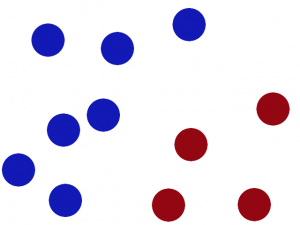
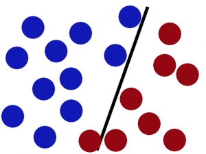
We have 2 colors of balls on the table that we want to separate.

svm1

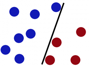
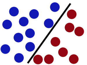
We get a stick and put it on the table, this works pretty well right?

svm2

Some villain comes and places more balls on the table, it kind of works but one of the balls is on the wrong side and there is probably a better place to put the stick now.

svm3

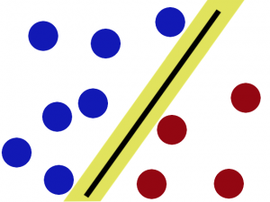
SVMs try to put the stick in the best possible place by having as big a gap on either side of the stick as possible.

svm4

Now when the villain returns the stick is still in a pretty good spot.

svm5

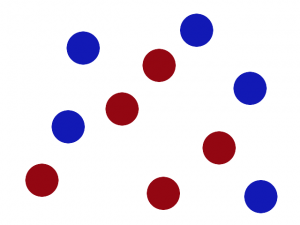
There is another trick in the SVM toolbox that is even more important. Say the villain has seen how good you are with a stick so he gives you a new challenge.

svm6

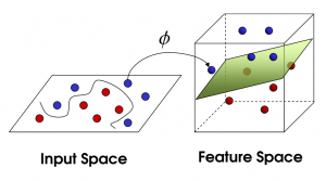
There’s no stick in the world that will let you split those balls well, so what do you do? You flip the table of course! Throwing the balls into the air. Then, with your pro ninja skills, you grab a sheet of paper and slip it between the balls.

svm7

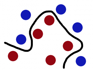
Now, looking at the balls from where the villain is standing, they balls will look split by some curvy line.

svm8

Boring adults the call balls data, the stick a classifier, the biggest gap trick optimization, call flipping the table kernelling and the piece of paper a hyperplane.


That was copperking’s explanation.

Related: Udi Aharoni created a video visualizing a polynomial kernel:


And, more recently, William Noble published a paper in Nature Biotechnology. You can access an expanded version here. Thanks to Mark Gerstein for tweeting this paper.


Happy kernelling!


Share and Enjoy:
  • Fark
  • Digg
  • Technorati
  • del.icio.us
  • StumbleUpon
  • Facebook
  • Reddit
  • Twitter
  • FriendFeed
  • PDF
  • email
  • Print
  • Google Bookmarks

Carnival of Evolution, February 2014 Edition

Wow, I haven’t posted anything in quite a while. Things are busy outside blogoland. But committing this blog to the February edition of the Carnival of Evolution just made me do it, so here goes. We’ll do this by scales, bottom up.

Molecular

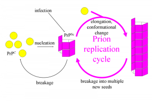
Prions are the infective agents that cause transmissible spongiform encephalopathies such as Mad Cow Disease in, well, cows, and Kuru or Kreuzfeldt-Jakob disease in humans.  Apparently prions are subject to natural selection — evolution — and as the Lab Rat reports, no DNA is required.

800px-Prion_Replication

Fibril model of prion propagation. Source: wikipedia

Back to genomes, can some genomes evolve more slowly than others? Larry Moran tackles this question in Sandwalk.

Microbial

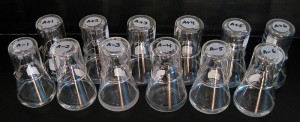
The E. coli long-term evolution experiment is an ongoing study in experimental evolution led by Richard Lenski that has been tracking genetic changes in 12 initially identical populations of asexual Escherichia coli bacteria since 24 February 1988. What have we learned? A meta-post linking to other posts summarizes five important things you can learn by looking at over 50,000 generations of bacterial evolution. Larry Moran discusses the unpredictability of evolution and potentiation in Lenski’s long-term evolution experiment.


800px-Lenski's_12_long-term_lines_of_E._coli_on_25_June_2008

The 12 evolving E. coli populations on June 25, 2008 Source: Wikipedia

Animal

A new book is out, The Monkey’s Voyage by Alan de Queiroz, and it is reviewed by Richard Conniff. How Did Monkeys Cross the Atlantic? A Near-Miraculous Answer was posted at strange behaviors. Speaking of monkeys, or rather apes, a comparative examination fo the chimp and human genomes reveal that 154 human genes have undergone positive selection compared with 233 chimp genes, after our phylogenetic split. Surprisingly, these are not the genes you may expect to have been selected as such.

From primates to canines, one dog has managed to outlive all others in its species… or its genes have. How? Read Carl Zimmer’s fascinating story on How A Dog Has Lived For Eleven Thousand Years posted at The Loom. In contrast, one species which is no longer with us is the Beelzebufu frog, also known as the Frog from Hell. Yes, this one ate dinosaurs, some 75 million years ago. Yikes.

As climate change continues to affect our world, species migrate and/or change phenotypes to adapt.  Or do they? Ben Haller recommends that you read Andrew Hendry’s post in Eco-Evo Evo-Eco to find out more.


Jump to 4:09 to see the Frog from Hell.

Mineral

How can you solve evolutionary problems with computers? A blog written by C. Titus Brown’s students explains evolutionary simulations and experiments in silico. While Bradly Alicea presents methods for Bet-hedging and Evolutionary Futures posted at Synthetic Daisies. A re-examination of Hamilton’s rule tells us why altruism is not only not rare as an evolutionary trait, it should probably be expected and quite frequent. Bjorn Ostman reports in Pleiotropy about Sewall Wright’s last paper on adaptive landscapes.


hedging-stocks-2

Bet-hedging as an investment strategy. Use a rowboat and a hang-glider.

While Titus’s students and others have been evolving things in computers, John Wilkins tackles the question whether life exists at all. No spoilers here, you will have to read it. You should probably also read Wilkins’s new book, on the Nature of Classification


That’s it! Thank you for being with us, a short post for a short month. Don’t forget to submit to the March carnival!


Share and Enjoy:
  • Fark
  • Digg
  • Technorati
  • del.icio.us
  • StumbleUpon
  • Facebook
  • Reddit
  • Twitter
  • FriendFeed
  • PDF
  • email
  • Print
  • Google Bookmarks

Science funding on other planets

Got this from a tweet by Casey Bergman


ipN0ExT

Share and Enjoy:
  • Fark
  • Digg
  • Technorati
  • del.icio.us
  • StumbleUpon
  • Facebook
  • Reddit
  • Twitter
  • FriendFeed
  • PDF
  • email
  • Print
  • Google Bookmarks

BOSC 2014 Guess the Keynote Competition

(From Peter Cock, via the OBF News Blog)


We’re pleased to officially confirm that one of the two keynote speakers
for the 15th annual Bioinformatics Open Source Conference (BOSC 2014) will
be C. Titus Brown, as he announced on Twitter recently:

Titus Brown (@ctitusbrown):
Excited to be a keynote speaker at BOSC 2014! My title:
“A History of Bioinformatics (in the year 2039)”
– plenty of room for mischief 😉
https://twitter.com/ctitusbrown/status/410934403565490176

In recognition of the growing use of Twitter and social media within science
as a way of connecting across geographical divides, we’re announcing a
Twitter competition to guess who is scheduled to give the second keynote
at BOSC 2014 in Boston.

To enter, please tweet using hashtag #bosc2014 and include us via @OBF_BOSC,
e.g.

I think @OBF_BOSC should invite “Professor X” to be a keynote speaker
at #BOSC2014 because…

The first correct entry (within one week) will be awarded one complementary
BOSC 2014 registration fee for themselves, or a nominated group member. This
does not cover travel or accommodation, and there is no cash substitute if you
cannot attend BOSC 2014. Members of the OBF board, BOSC organizing
committee, and ISMB SIG committee are not eligible, nor are the keynote
speakers themselves.

We intend to announce the mystery keynote speaker and any Twitter competition
winner in one week’s time, but reserve the right to cut short, modify, or
cancel the competition.

Our ulterior motive is to crowd source ideas for future keynote speakers in
BOSC 2015, so some serious suggestions please

Further details about BOSC 2014 will be posted here:
http://www.open-bio.org/wiki/BOSC_2014

Thank you,

Peter Cock & Nomi Harris, BOSC 2014 co-chairs.

This was also posted to the OBF News Blog,
http://news.open-bio.org/news/2013/12/bosc-2014-keynote-competition/

BOSC and the OBF are on Twitter as:
https://twitter.com/OBF_BOSC
https://twitter.com/OBF_news

Share and Enjoy:
  • Fark
  • Digg
  • Technorati
  • del.icio.us
  • StumbleUpon
  • Facebook
  • Reddit
  • Twitter
  • FriendFeed
  • PDF
  • email
  • Print
  • Google Bookmarks